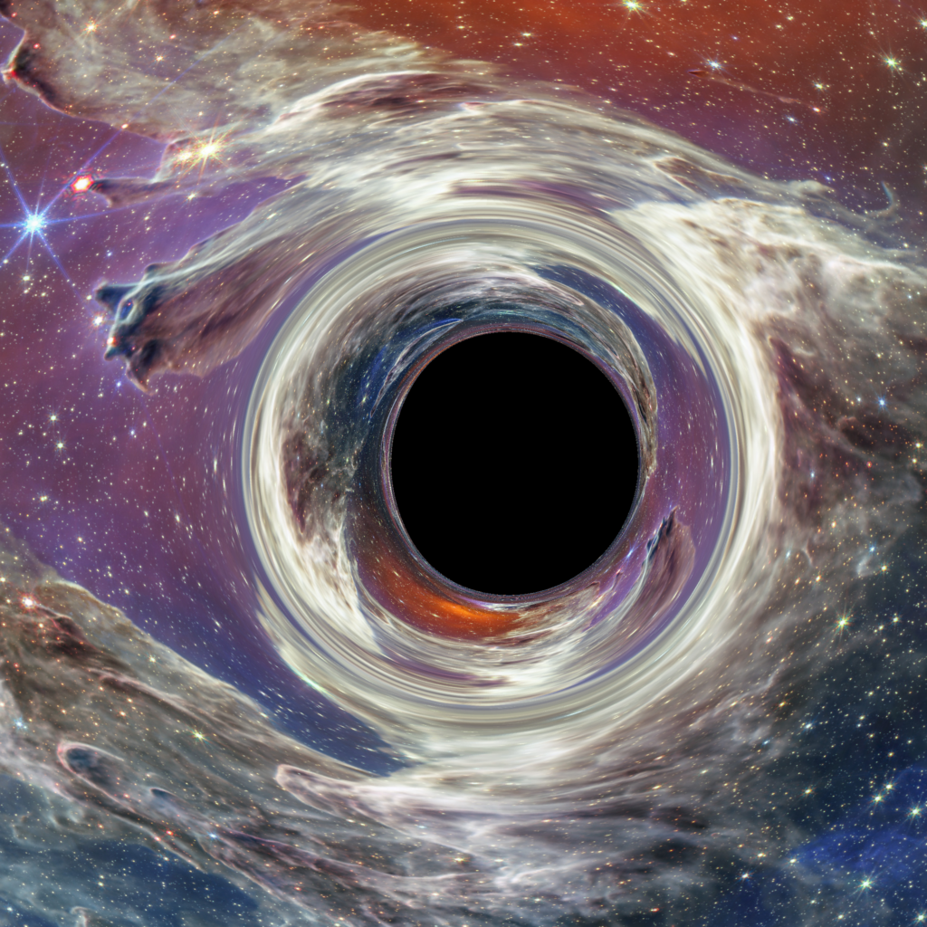
This page is a deep dive into the second part of the Black Hole Shadows project. The first part was an experiment: Claude Code organized my old research code from one prompt. After that pass, I wanted to improve further the code.
The biggest change is an optional GPU backend for Apple Silicon. It traces the light rays 20 to 60 times faster than the CPU using 8 cores. A 2048 × 2048 image (more than 4 million rays) now takes 6 to 11 seconds on a MacBook. This page explains how the GPU port works, how fast and how accurate it is, and the smaller improvements that came with it.
What changed after the first pass
The first pass made the code readable again. The follow-up work made it a tool. The main changes were
- GPU support on Apple Silicon, so renders run much faster
- better formats for the saved files, so each run stays compact and easy to find
- support for multiple sky backgrounds, so the same black hole can be rendered against different scenes.
Why ray tracing suits a GPU
The tracer sends one light ray for each pixel. Each ray is computed independently. This is the type of work that a GPU does well: many small, identical tasks at the same time.
But the rays do not take the same time. The integrator (RKF45) uses an adaptive step. A ray far from the Black Hole takes large steps and ends quickly. A ray near the photon ring takes many small steps. Some rays fall in, some hit the disk and some escape.
This difference decides the design:
- Array operations are not a good fit. MLX has NumPy-style arrays. With arrays, all rays move one step together, so all rays wait for the slowest ray at each step.
- A custom kernel is a good fit. One GPU thread traces one ray. Each thread has its own step size and its own stop condition, and it stops when its ray ends.
- Numba cannot do it on a Mac. The CPU code uses numba, but numba GPU support is for NVIDIA (CUDA) only.
So each tracer (Kerr and Weyl) got one kernel in the Metal Shading Language (MSL), the C++-based language of Apple GPUs. MLX compiles it at run time with mx.fast.metal_kernel. The kernel is a port of the numba functions: metric, Christoffel symbols, geodesic equations, RKF45 step and initial ray state.
The float32 problem
Apple GPUs do not support float64. The kernels use float32, which keeps approximately 7 significant digits instead of 16. The numba code was written for float64, so a direct copy was not possible. These are the changes:
- Step-size floor. In float32, a step smaller than 1e-5 does not change the state. The GPU uses this value as the smallest step.
- Limits. Each ray has a maximum number of steps, and each step has a maximum number of retries. The CPU has no limits, but on the GPU a ray that does not end blocks the launch.
- Status 3 and CPU fallback. A ray that reaches a limit, or that gets a NaN or Inf value, gets status 3 (failed). After the launch, the runner traces these pixels again on the CPU, in float64. Thus the final image does not depend on float32 for the difficult rays.
- Derivatives. The CPU calculates some derivatives with a central difference (step 1e-6). In float32, that step gives only noise. The GPU uses analytic derivatives for the Schwarzschild part and a scaled step for the disk part.
- The kink at the disk. The disk potential has a kink at z = 0. A central difference across the kink gives a wrong value, so near the disk plane the GPU uses a one-sided difference.
How the GPU run works
- The runner selects the device from the config (
[tracer] device) or the command line (--device gpu). If MLX or an Apple GPU is not available, it logs a warning and uses the CPU. - The CPU calculates the observer constants once, in float64, and sends them to the kernel.
- For the Weyl case, the CPU builds or loads the lambda lookup table, and the GPU only reads it. This is because the table uses scalar adaptive quadrature (
scipy.quad), not supported by the GPU. - The runner sends the image rows to the GPU in chunks of 32 rows. Each chunk is one kernel launch.
- Each thread traces its ray with RKF45 and writes the end state and a status code.
- The runner traces the status-3 pixels again on the CPU and writes the GPU statistics to
run.json.
Note: Why chunks 32 rows?
macOS can stop a GPU launch that runs too long (a watchdog).
Apple does not document the limit, so the code uses a budget of 1 s for each launch.
In a pessimistic scenario, a 32-row launch for a 1000s x1000s image takes less than 1 second.
The first launch in each process compiles the kernel (0.2 to 0.9 s). Later launches use a cache.
How fast it is
| Case | CPU (numba, float64) | GPU (MLX, float32) | Speedup |
|---|---|---|---|
| Schwarzschild with disk | 1.82 s | 0.079 s | 23× |
| Schwarzschild, no disk | 1.90 s | 0.063 s | 30× |
| Kerr, a = 0.9 | 0.81 s | 0.019 s | 43× |
Apple Silicon, 64 × 64 pixels, median of 3 warm runs, lookup table already cached. A cold start (first trace, with compile) takes 4 to 6 s on the CPU and 0.2 to 0.9 s on the GPU.
The small benchmark is the fair comparison. The real gain is at large sizes. With the GPU, a 2048 × 2048 Kerr image takes 6 to 11 seconds from start to end. The lower time is a run where all rays finish on the GPU. In the slower runs, 8 to 14 rays of more than 4 million fail in float32, and their CPU re-trace adds about 3 seconds.
Is the GPU result correct?
The CPU (numba, float64) stays the reference. The tests in tests/test_gpu_backend.py compare the two devices:
- Kerr, a = 0.9, 64 × 64: 0 of 4096 pixels changed class. The relative error of the geodesic equations is approximately 1e-6.
- Schwarzschild with disk (M = 0.9, MD = 0.1), real lookup table: 0 of 4096 pixels changed class, and 1140 pixels hit the disk on both devices. The median difference in the end coordinates is approximately 5e-4.
- Fallback: no pixel needed the CPU re-trace in these benchmark runs.
Pixels very near the shadow edge can change class in float32. For reference results, use the CPU.
How to use it
uv sync --extra gpu
 uv run bh-shadow configs/kerr_a0.9_nodisk.toml --device gpu
 uv run bh-shadow configs/schwarzschild_disk.toml --n 64 --device gpu
The default device auto still selects the CPU. All measured speedups are above 1.5×, so the next step is to let auto select the GPU.
Other improvements
One command, one config. Each run is a TOML file with the spacetime (M, a, MD), the observer, the tracer and the plot.
Each run gets its own folder with a run.json that records the parameters, versions, threads and times. A progress bar shows the trace.
Smaller, faster files. The lambda lookup table was a text file. Now it is a compressed NumPy file: 37.4 MB → 10.8 MB, and it loads in 0.04 s instead of 0.23 s. The code builds the table once and reuses it for the same parameters. The run outputs are one compressed outputs.npz file instead of many text files.